
WP3: Inverse modelling of the coupled COS and CO2 budgets
Activity 3.1: Implement COS & isotopologues in TM5 4D-Var system
The basis for this activity will be the TM5-4DVar system for CO2 [Basu et al., 2014; Pandey et al., 2016]. In short, this model version assimilates surface observation of CO2 to optimise grid scale exchange of CO2 with the biosphere and the ocean, a process known as source optimisation. This mathematical procedure is generally called “inverse modelling”, and involves in the case of 4DVar the use of an adjoint model [Tarantola, 2005; Krol et al., 2008]. The TM5-4DVar system is flexible in the sense that (i) sources and sinks can be optimised on flexible time intervals (ii) different categories can be optimised (e.g. ocean, biosphere) (iii) next to surface observations, also aircraft-data and/or satellite-derived atmospheric columns can be assimilated (iv) bias correction can be applied to account for biases in certain measurement information [Houweling et al., 2014]. TM5-4DVar is also “multi-tracer”, which implies that sources and sinks of different compounds can be optimised using observations of these compounds [Pandey et al., 2016].
Activity 3.2: Joint COS & CO2 inversion using surface observations
This activity will use surface observations of COS and CO2 from the NOAA/ESRL network [Montzka et al., 2007] to constrain sources and sinks of CO2 and COS. Starting point will be earlier inversion studies [e.g. Berry et al., 2013], which showed that largest uncertainties are associated with tropical ocean sources and biosphere uptake. The TM5-4DVar framework (Activity 3.1) simulates all individual observations and estimates an error for the model-data mismatch [Bergamaschi et al., 2010]. I will start with a state vector that consists of (i) monthly values of GPP calculated by SiB4, translated into CO2 and COS uptake fluxes (ii) respiration fluxes of CO2 calculated by SiB4 (iii) Land–atmosphere exchange fluxes of COS (Activity 1.1) (iv) oceanic emissions of COS [Launois et al., 2015b] and biomass burning emissions. In fact, a very-similar set-up has recently be recommended to derive GPP information [Launois et al., 2015a]. Technically, to optimise fluxes, monthly time-series of hourly exchange fluxes are multiplied with scaling factors that are allowed to vary per month and grid cell (with further constraining spatial and temporal correlations). To illustate the idea, the figure shows preliminary results from an inversion over the USA using the WRF-Stilt system, coupled to SiB4.
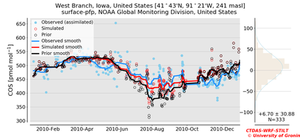
(Ivar van der Velde, personal communication). Preliminary results from an inverse modelling system, employed over the USA domain. The system uses the coupled CO2 and COS biosphere model SiB4 and WRF-Stilt for atmospheric transport. Non-optimised (black) modelled COS mixing ratios are brought closer to observations (blue) by optimising parameters related to the biosphere (red).
Activity 3.3: COS budget estimate using additional COS data from satellites, AirCore & isotope sampling program
In this integrating activity, I will additionally use the measurements performed in WP2, together with satellite measurements, to better constrain the joint atmospheric COS and CO2 budgets.
Since surface observations are likely sensitive mostly to surface processes influencing the COS mixing ratios, the target here to include measurements that also inform about stratospheric breakdown of COS. Stratosphere–troposphere exchange transports COS to the stratosphere through the tropical tropopause layer (TTL), and transports stratospheric air back to the troposphere through tropopause folds and large scale polar subsidence. The modelled COS profile shape will be sensitive to these processes but also to COS photolysis above roughly 20 km altitude. Apart from assimilation of surface data, I will therefore use AirCore, high altitude COS samples, and satellite measurements to obtain information about the stratospheric COS budget in a 4D-Var setup. Apart from measurements from WP2, I will use satellite data from the TES satellite (since 2004, upper troposphere) [Kuai et al., 2014; 2015], ACE (upper troposphere, lower stratosphere, since 2004) [Barkley et al., 2008; Velazco et al., 2011], and MIPAS (upper troposphere, lower stratosphere, 2002-2012) [Brühl et al., 2015; Glatthor et al., 2015]. Together with surface constraints (Activity 3.2) assimilation of these observations will lead to “optimised” COS simulations that provide the best possible estimate of the stratospheric and tropospheric COS budget.